---
title: "Scientific Maps Analysis with the `R` package `bibliometrix`"
date: 09-09-2022
description: "Example of scientific maps for bibliometric analysis"
image: graph.png
categories:
- bibliometry
- mapping
- bibliometric analysis
format:
html
#code-fold: show
doi: 10.5281/zenodo.10079724
citation: true
---
```{r include=FALSE}
# Installation of some useful packages
if(!isTRUE(require("prettydoc"))){install.packages("prettydoc")}
if(!isTRUE(require("rio"))){install.packages("rio")}
library(prettydoc)
library(rio)
```
      
# Introduction
# Bibliographic Data
The bibliographic data are based on the search query that has been made. For the moment we have focused on one of the lines of the [SEJ670](/now/index.qmd) UCO Research Group, **neophilia/neophobia in tourism**. Needles to say that it would be applied to other research lines; however, watch out when filtering and redefining the database because we have to remove areas that are not of our interest, for example, in our selection there were references about zoology, biology, etc..., given that there is also neophilia and neophobia, especially the latter, specifically in animals, well, we must be careful because some area can sneak in the form of journals and references not related to our research area.
**Data source**: Clarivate Analytics Web of Science (<http://apps.webofknowledge.com>)
**Format**: Bibtex
**Query**: "Web of Science Core Collection"
**Range**: 1995-2022
**Document type**: All
**Query date**: September, 2022
# Package installation, data loading and conversion
As the objective is to see what analysis the tool does and how it does it, the steps of installation, data loading and conversion have been omitted, although it is an important step since it must be done in `R`, after downloading the data from WoS or Scopus, which also has its own technique. After a lot of research we managed to find a way to merge both databases and it works perfectly, and it also automatically omits duplicate references. **With this procedure we can have both databases in a single file and although WoS has more references (as a general rule, although not always), Scopus almost always has some different one/s and even if they are few, at least we practically cover the two most important sources of articles.** It is worth mentioning that in the last updates of this `Bibliometrix` package other open bibliographic databases such as _OpenAlex_, _Dimensions_, _Lens_, and from the medical field such as _PubMed_ and _Cochrane_ have been included.
```{r load bibliometrix, message=FALSE, include=FALSE}
# Stable version from CRAN (Comprehensive R Archive Network)
# if you need to execute the code, remove # from the beginning of the next line
# install.packages("bibliometrix")
# Most updated version from GitHub
# if you need to execute the code, remove # from the beginning of the next lines
# install.packages("devtools")
# devtools::install_github("massimoaria/bibliometrix")
library(bibliometrix)
```
```{r Data loading, warning=FALSE, include=FALSE}
# Convertimos el fichero obtenido de WoS en un dataframe bibliográfico con R
wos <- convert2df("wos.bib", dbsource = "wos", format = "bibtex")
```
# 1. Descriptive Analysis
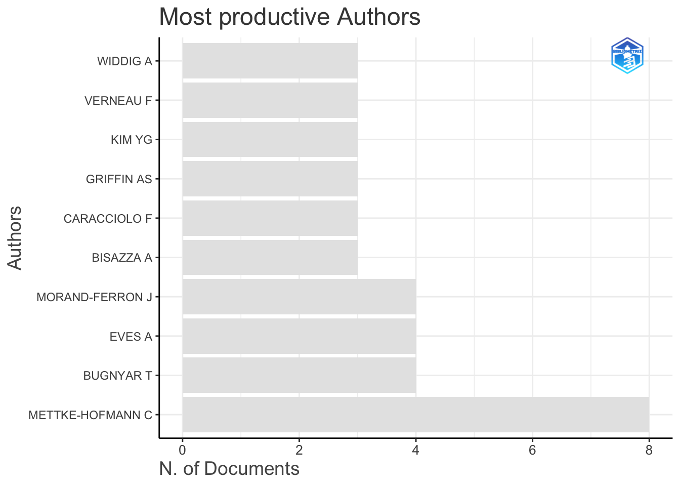
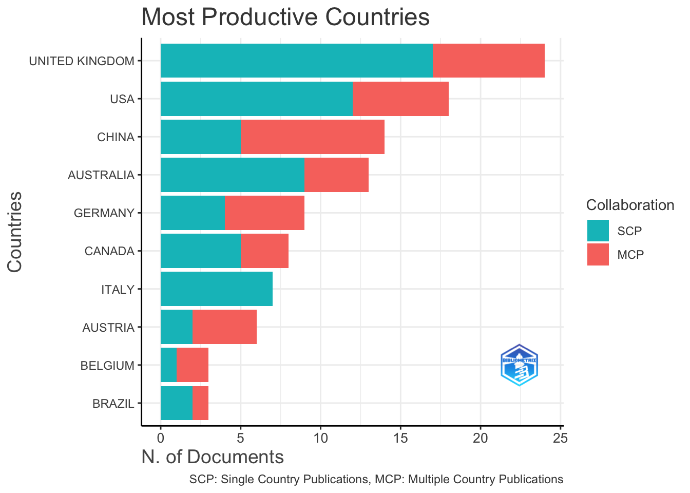
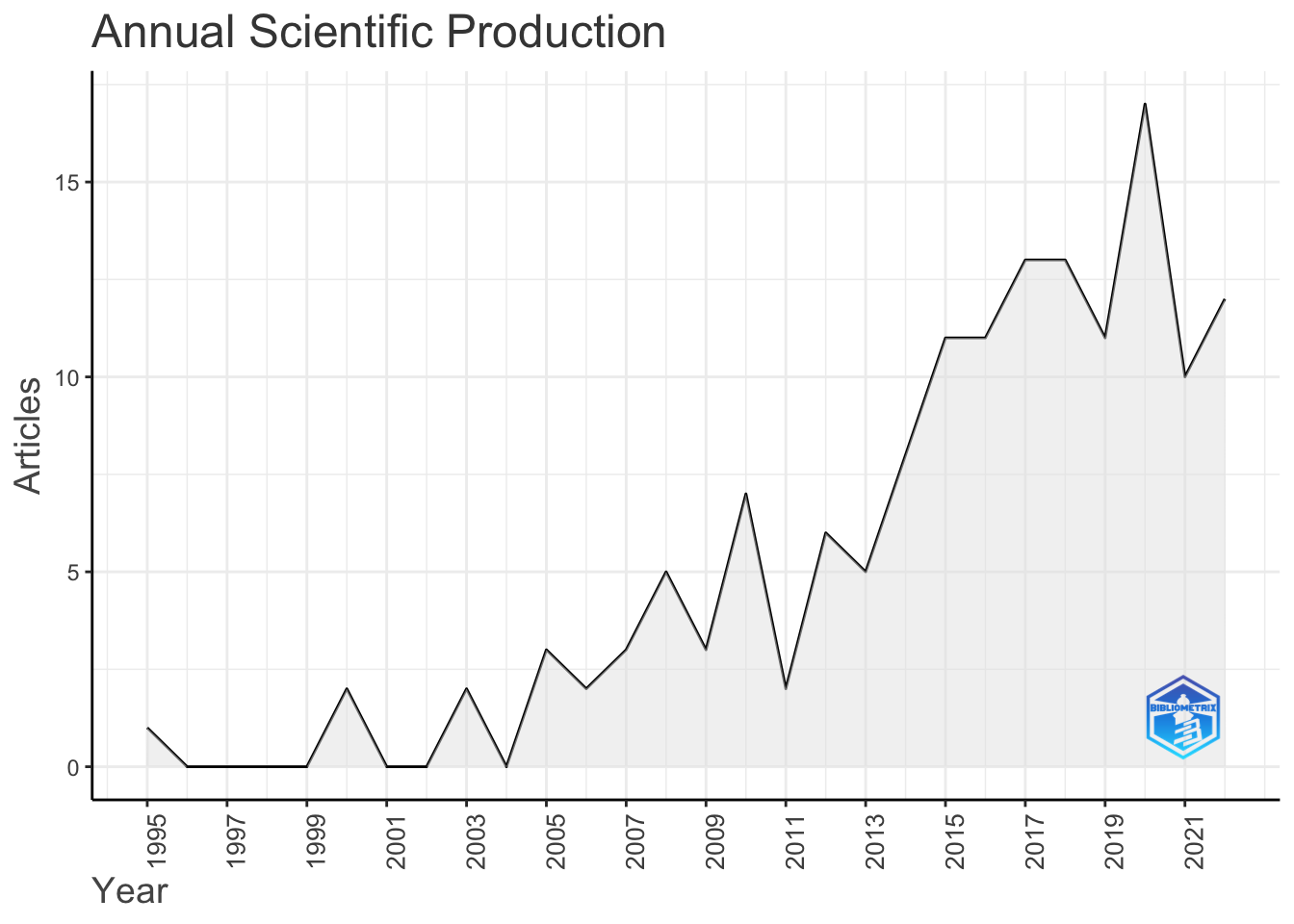
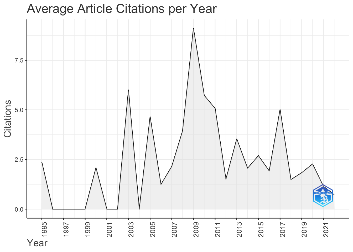
The descriptive analysis of the package provides a lot of information on the annual development of research, the most productive $k$ authors, articles, countries and relevant keywords.
## 1.1. Main findings on the database analysed
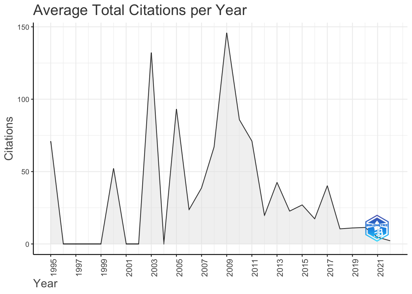
The following table shows a summary of the data and other interesting classifications: _n_umber of authors_, _number of documents_, _scientific production for each year_ (and its average growth), the _most productive authors_, the _countries_ and the _corresponding citations_, the _most relevant journals_, the _most relevant keywords_, etc...
Moreover, this information can also be obtained in graphs.
```{r Descriptive Analysis, echo=FALSE, comment=NA}
#options(width=160)
results <- biblioAnalysis(wos)
summary(results, k=10, pause=F, width=130)
plot(x=results, k=10, pause=F)
```
## 1.2. Most cited references
We can also obtain the most cited references and their number:
```{r Most cited references, echo=FALSE, comment=NA}
CR <- citations(wos, field = "article", sep = ";")
cbind(CR$Cited[1:20])
```
# 2: Co-citation analysis structure
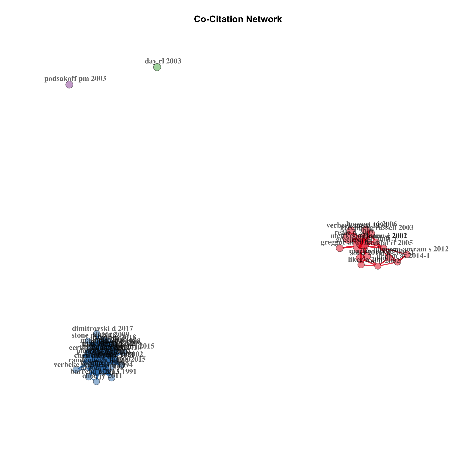
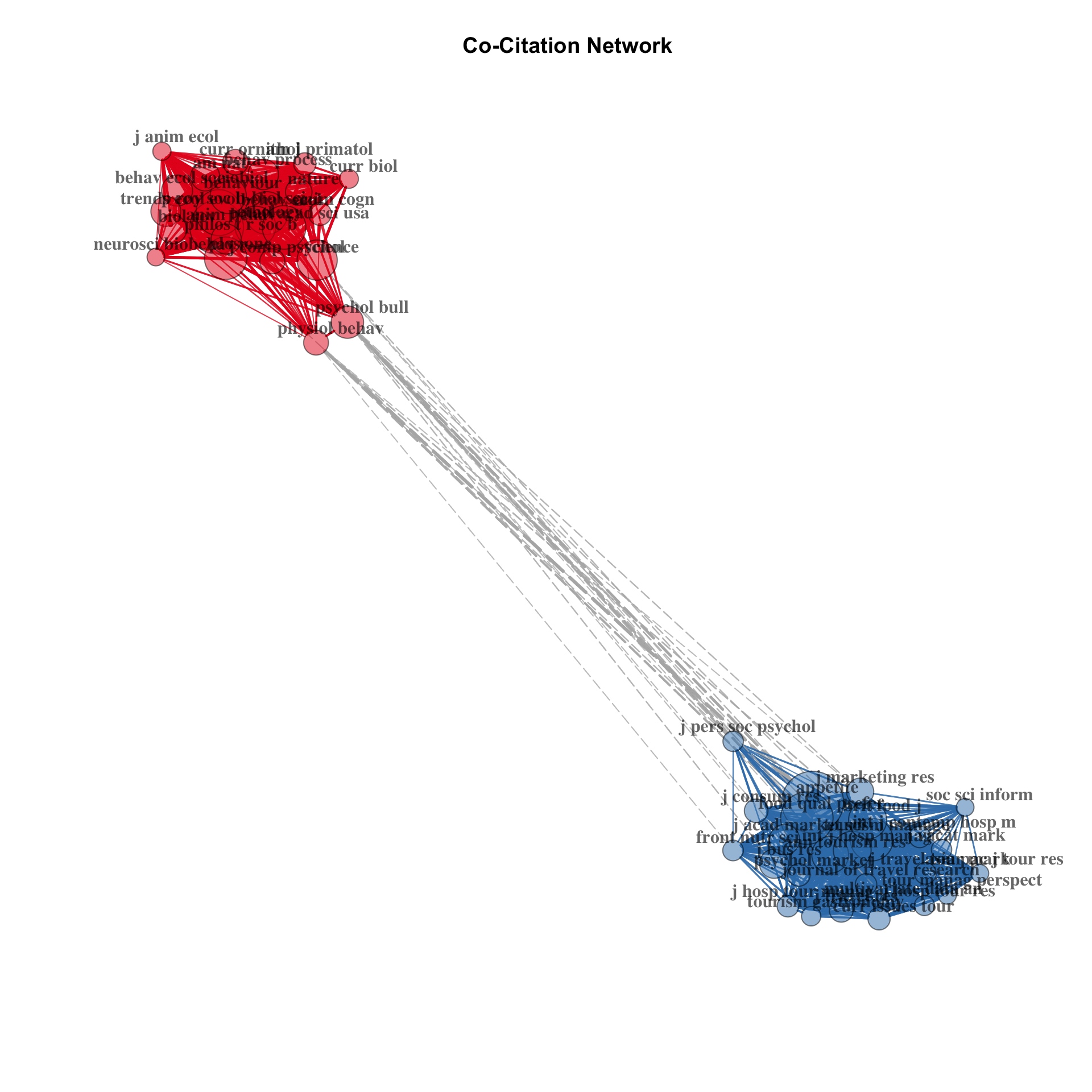
Citation analysis is another remarkable tool of the bibliometric analysis offered by the package. It shows the structure of a specific field through the links between nodes (e.g. authors, articles, journal). The interesting option is that the edges can be interpreted differently depending on the type of network, i.e. co-citations, direct citations, bibliographic linking, etc.... This is very useful and can be exploited quite a lot.
Below we have taken the three standard examples shown in the original reference but adapted them to our database.
_First_, a co-citation network showing the relationships between the cited-referred works (nodes).
_Second_, a co-citation network that uses the cited journals as the unit of analysis.
The dimensions useful for commenting on co-citation networks are: **(i)** centrality and peripherality of nodes, **(ii)** their proximity and distance, **(iii)** strength of links, **(iv)** clusters, **(v)** bridging contributions.
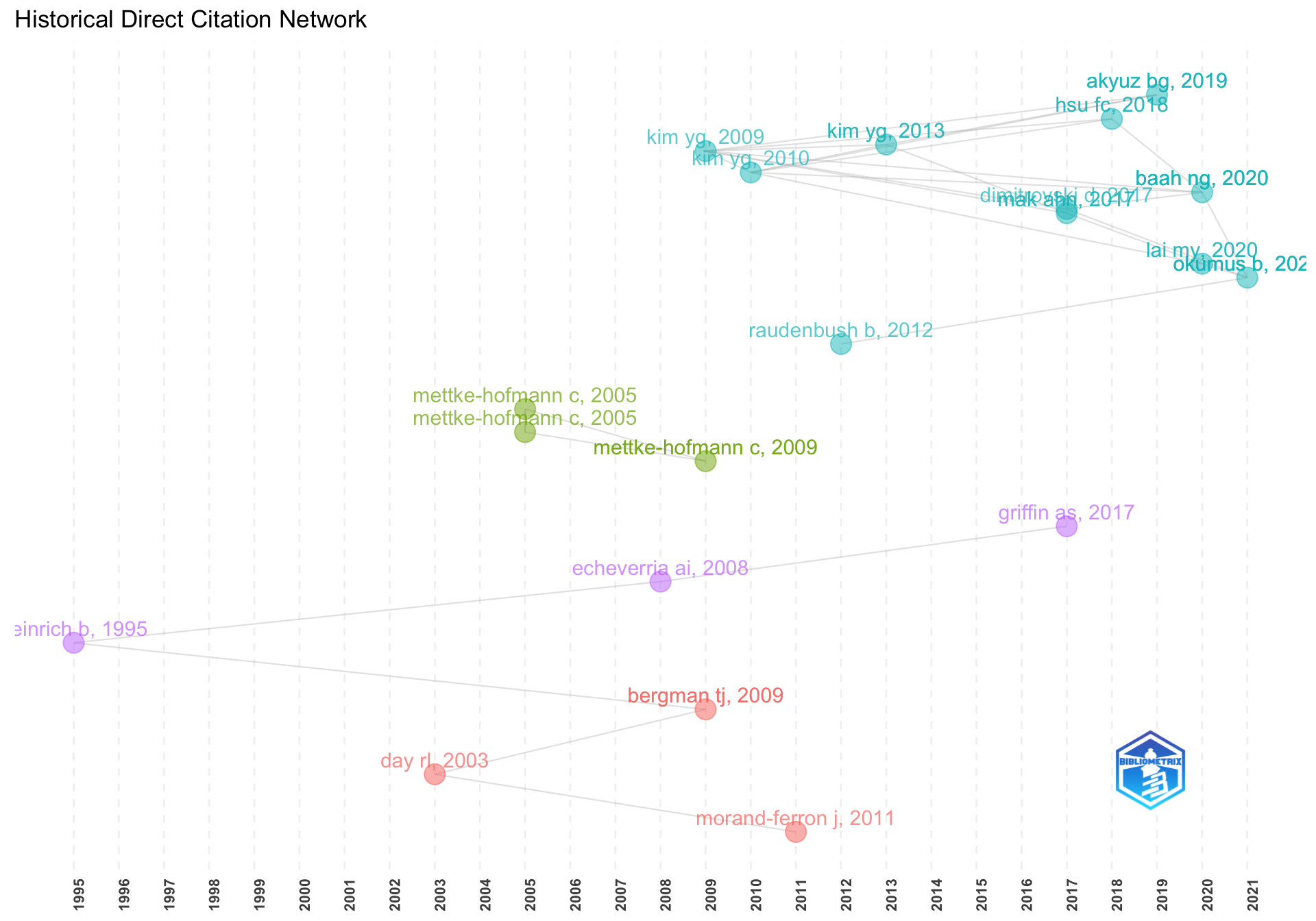
_Third_, a historiography that is built on direct quotations. It traces the intellectual links in a historical order. The cited works of thousands of authors contained in a collection of published scientific articles are sufficient to reconstruct the historiographical structure of the field, pointing out the basic works in it.
## Analysis of co-citations of articles (references)
This is the typical _VosViewer_ graph, in this case for a visualization of the co-cite network. The graph parameters have not been modified to make it clearer but the **graph options** shown below are mainly for visual fine tuning. Without seeing the code this may be useless but it is interesting to know that it can be tweaked and made more readable. The interesting thing would be to be able to eliminate those co-citations that appear isolated and focus only on those where there are relationships.
- `n = 50` (this function traces the top 50 cited references)
- `type = "fruchterman"` (the network layout is generated by the [Fruchterman-Reingold algorithm](https://github.com/gephi/gephi/wiki/Fruchterman-Reingold), there is the option of other types of algorithms, although I have not tested them and I do not know if they would work for us)
- `size.cex = TRUE` (the size of the vertices is proportional to its degree)
- `size = 20` (maximum size of the vertices)
- `remove.multiple = FALSE` (multiple edges are not eliminated, the opposite is `TRUE`)
- `labelsize = 1` (defines the size of the vertices labels)
- `edgesize = 10` (the thickness of the edges is proportional to their strength. `Edgesize` defines the maximum value of the thickness)
- `edges.min = 5` (only traces edges with a force greater than or equal to 5)
- all other arguments assume default values.
```{r Co-citation network, echo=FALSE, fig.height=10, fig.width=10, comment=NA}
NetMatrix <- biblioNetwork(wos, analysis = "co-citation", network = "references", sep = ";")
net=networkPlot(NetMatrix, n = 50, Title = "Co-Citation Network", type = "fruchterman", size.cex = TRUE, size = 20, remove.multiple = FALSE, labelsize = 1, edgesize = 10, edges.min = 5)
```
```{r Co-citation net stat, eval=FALSE, comment=NA, include=FALSE}
# El cuadro resumen Análisis descriptivo de las características de la red de citación de artículos
# netstat <- networkStat(NetMatrix)
#summary(netstat,k=10)
```
## Analysis of journal co-citations (source)
```{r Co-citation source network, comment=NA, fig.height=10, fig.width=10}
wos=metaTagExtraction(wos,"CR_SO",sep=";")
NetMatrix <- biblioNetwork(wos, analysis = "co-citation", network = "sources", sep = ";")
net=networkPlot(NetMatrix, n = 50, Title = "Co-Citation Network", type = "auto", size.cex=TRUE, size=15, remove.multiple=FALSE, labelsize=1,edgesize = 10, edges.min=5)
```
Descriptive analysis of the characteristics of the journal citation network.
This analysis is similar to the previous one but with journal citations.
```{r So Co-citation net stat, echo=FALSE, comment=NA}
netstat <- networkStat(NetMatrix)
summary(netstat,k=10)
```
# 3: Historiography - Direct citation links
This analysis provides us with direct citation links by author and year, which is interesting to see who cites whom and when.
```{r Direct citation network, echo=FALSE, fig.height=10, fig.width=10}
histResults <- histNetwork(wos, sep = ";")
```
```{r Historiograph, echo=FALSE, fig.height=7, fig.width=10, comment=NA}
options(width = 130)
net <- histPlot(histResults, n=20, size = 5, labelsize = 4)
```
# 4: Conceptual structure - Co-word analysis
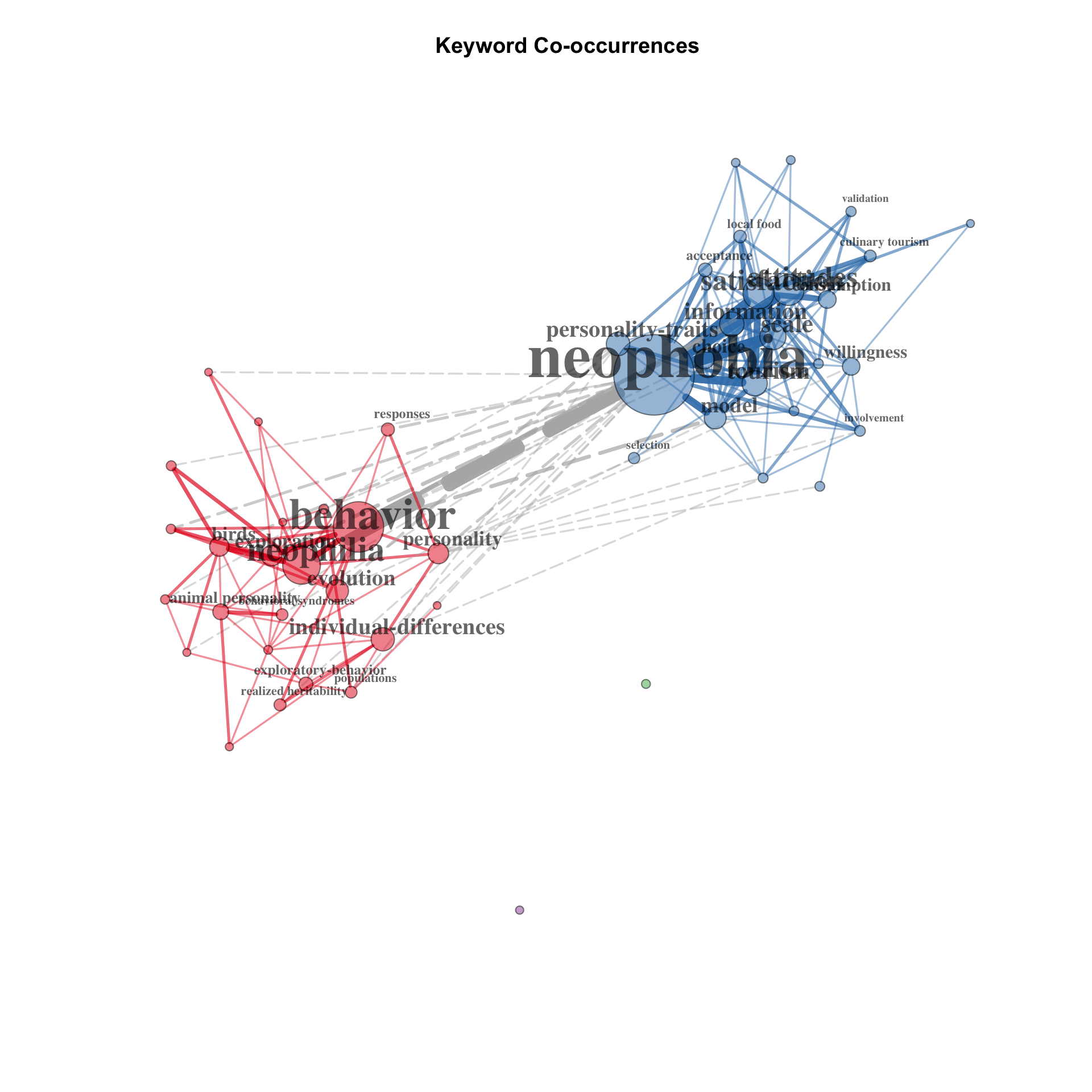
Co-Word Networks show the conceptual structure, which uncovers the links between concepts through co-occurrences of terms.
The conceptual structure can be used to understand the topics being discussed (research front) and to identify which are the most important and most recent topics.
The tool divides the whole time span into different periods and compares the conceptual structures which is useful to analyze the evolution of the topics over time.
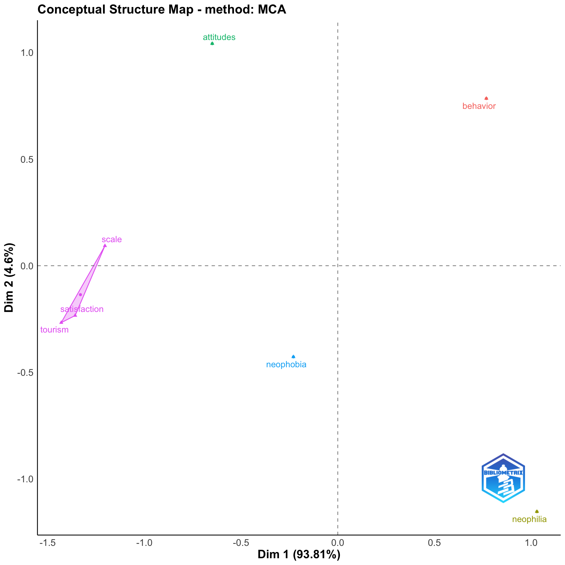
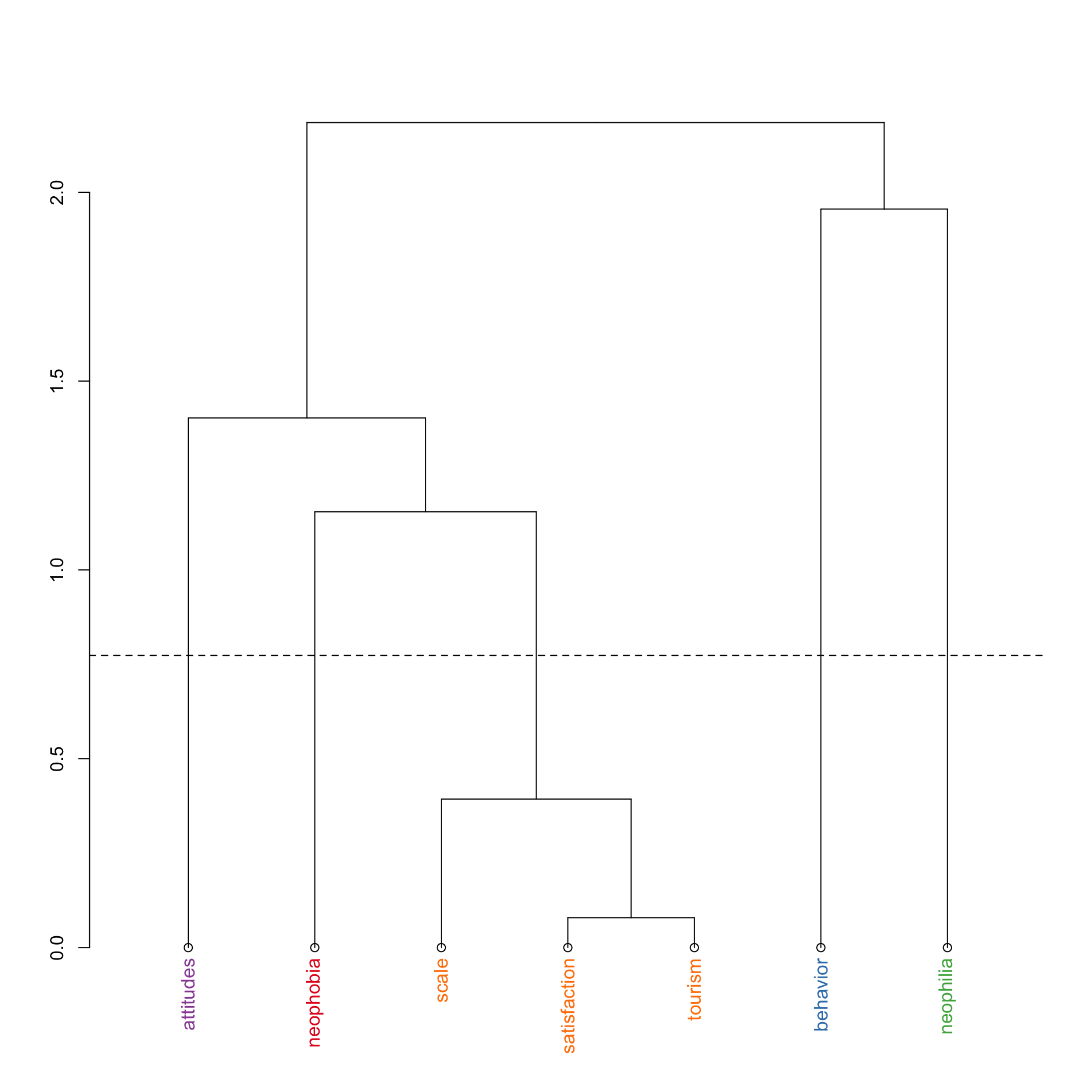
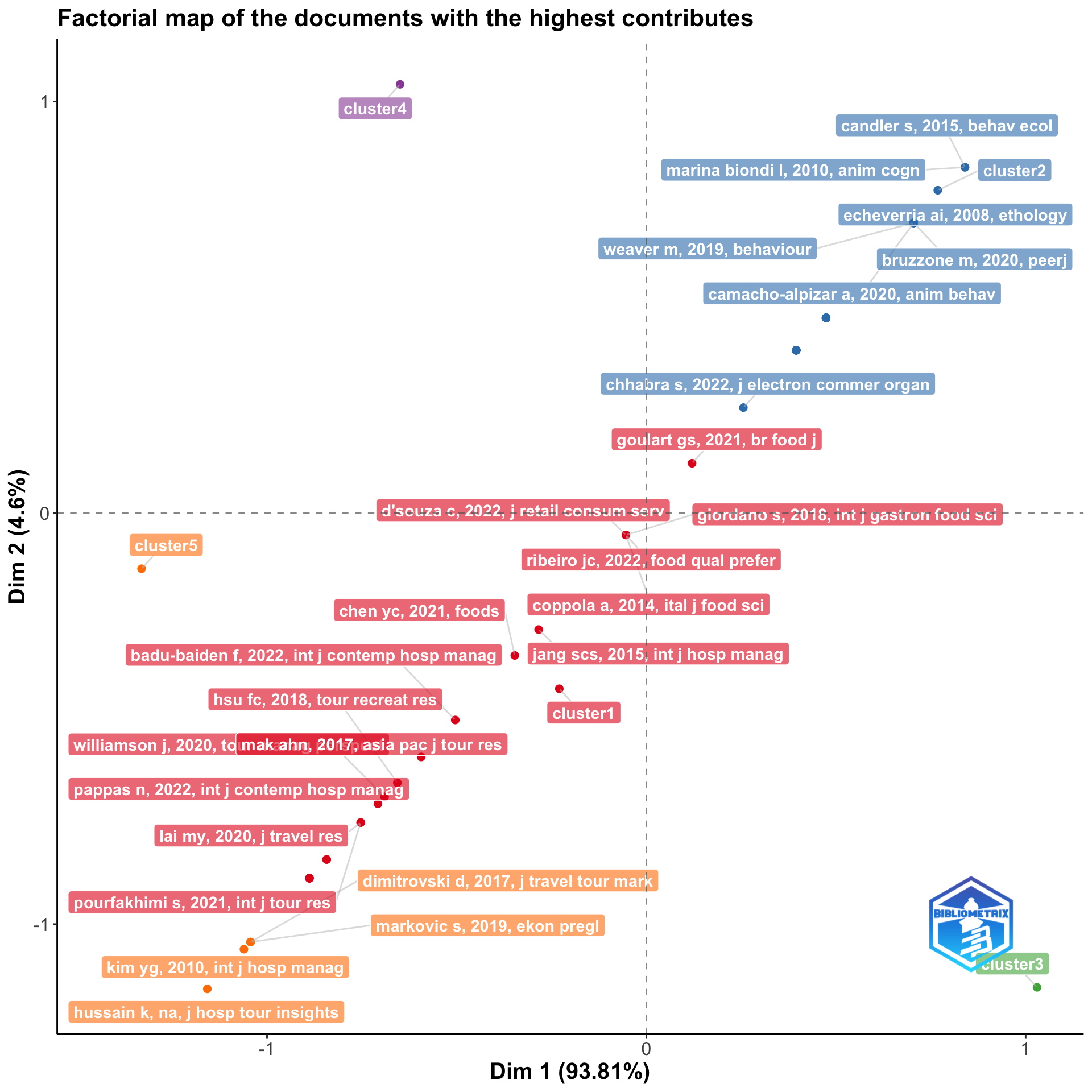
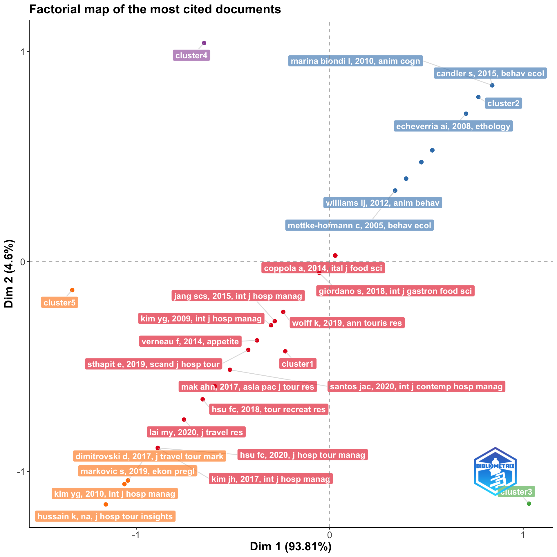
The package is able to analyze keywords, but also terms in article titles and abstracts. It does this by means of network analysis or correspondence analysis (CA) or multiple correspondence analysis (MCA). CA and MCA visualize the conceptual structure in a two-dimensional graph, which I also show below.
## Joint word analysis using keyword co-occurrences
As with the previous graph, the **options** are to make the graph more readable:
- `normalize = "association"` (the vertex similarities are normalized using association strength)
- `n = 50` (the function traces the top 50 cited references)
- `type = "fruchterman"` (The network trace is generated using the _Fruchterman-Reingold_ algorithm)
- `size.cex = TRUE` (the size of the vertices is proportional to their degree)
- `size = 20` (maximum size of the vertices)
- `remove.multiple = FALSE` (multiple edges are not removed)
- `labelsize = 3` (defines the maximum size of the vertices labels)
- `label.cex = TRUE` (size of vertices labels is proportional to their degree)
- `edgesize = 10` (thickness of the edges is proportional to their degree. `Edgesize` defines the maximum value of the thickness)
- `label.n = 30` (labels are drawn only for the top 30 vertices)
- `edges.min = 25` (Only plot edges with a strength greater than or equal to 25)
- all other arguments assume default values.
```{r Keyword co-occurrences, comment=NA, fig.height=10, fig.width=10}
NetMatrix <- biblioNetwork(wos, analysis = "co-occurrences", network = "keywords", sep = ";")
net=networkPlot(NetMatrix, normalize="association", n = 50, Title = "Keyword Co-occurrences", type = "fruchterman", size.cex=TRUE, size=20, remove.multiple=F, edgesize = 10, labelsize=5,label.cex=TRUE,label.n=30,edges.min=2)
```
```{r Keyword net stat, eval=FALSE, comment=NA, include=FALSE}
# Descriptive analysis of keyword co-occurrences network characteristics
# netstat <- networkStat(NetMatrix)
# summary(netstat,k=10)
```
## Joint word analysis by means of correspondence analysis
```{r Co-word Analysis, fig.height=10, fig.width=10}
suppressWarnings(
CS <- conceptualStructure(wos, method="MCA", field="ID", minDegree=15, clust=5, stemming=FALSE, labelsize=15,documents=20)
)
```
# 5: Thematic maps
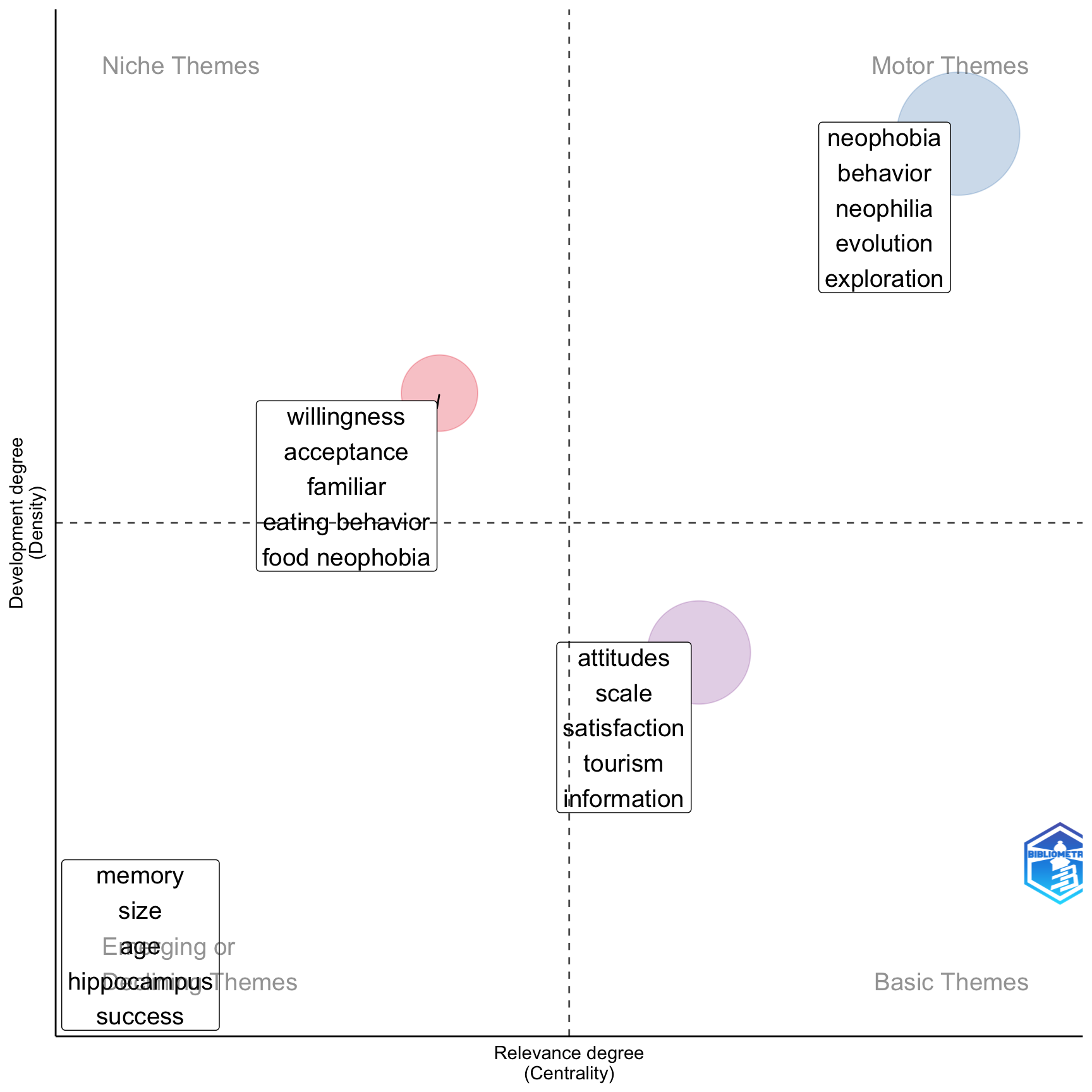
The co-word analysis draws clusters of the keywords. Themes are considered, whose density and centrality can be used to classify the themes and draw a two-dimensional diagram.
The thematic map is a very intuitive diagram and we can analyze the topics according to the quadrant in which they are placed: *(1)* upper right quadrant: *main topics* (as qualified by the authors of the tool); *(2)* lower right quadrant: **basic topics**; *(3)* lower left quadrant: **emerging or disappearing topics**; *(4)* upper left quadrant: **very specialized/niche topics**.
El análisis de co-palabras dibuja clusters de las palabras clave. Se consideran temas, cuya densidad y centralidad pueden utilizarse para clasificar los temas y trazar un diagrama bidimensional.
```{r ThematicMap, echo=TRUE, fig.height=9, fig.width=9}
Map=thematicMap(wos, field = "ID", n = 250, minfreq = 4,
  stemming = FALSE, size = 0.7, n.labels=5, repel = TRUE)
plot(Map$map)
```
The description of the cluster can then be requested from the program:
```{r}
Clusters=Map$words[order(Map$words$Cluster,-Map$words$Occurrences),]
library(dplyr)
CL <- Clusters %>% group_by(.data$Cluster_Label) %>% top_n(5, .data$Occurrences)
CL
```
# 6: Social structure - Collaboration analysis
This last section is also interesting. Collaborative networks show how authors, institutions (e.g., universities or departments) and countries relate to others in the field we are analyzing, in this case neophilia/neophobia in tourism. For example, the first figure below is a “Co-author network”. It uncovers regular study groups, hidden groups of scholars and key authors. The second figure is called an “Educational Collaboration Network” and uncovers relevant institutions in a specific research field and their relationships.
## Author collaboration network
```{r, Au collaboration network, fig.height=10, fig.width=10}
NetMatrix <- biblioNetwork(wos, analysis = "collaboration",  network = "authors", sep = ";")
net=networkPlot(NetMatrix,  n = 50, Title = "Author collaboration",type = "auto", size=10,size.cex=T,edgesize = 3,labelsize=1)
```
```{r Au coll stat, eval=FALSE, comment=NA, include=FALSE}
# Análisis descriptivo de las características de la red de colaboración de los autores
# netstat <- networkStat(NetMatrix)
# summary(netstat,k=15)
```
## Educational collaboration network
```{r, Edu collaboration network, fig.height=10, fig.width=10}
NetMatrix <- biblioNetwork(wos, analysis = "collaboration",  network = "universities", sep = ";")
net=networkPlot(NetMatrix,  n = 50, Title = "Edu collaboration",type = "auto", size=4,size.cex=F,edgesize = 3,labelsize=1)
```
```{r Edu coll stat, eval=FALSE, comment=NA, include=FALSE}
# Análisis descriptivo de las características de la red de colaboración educativa
# netstat <- networkStat(NetMatrix)
# summary(netstat,k=15)
```
## Collaboration network between countries
Finally, we can also obtain a graph of the collaboration network between countries, which can be useful to see between which countries there is more collaboration on the topic in question. For example, it can be seen that the country that has the most relationships is the United Kingdom. Spain, on the other hand, establishes collaborations with Japan, South Africa, Indonesia, Germany and China.
```{r, Co collaboration network, fig.height=10, fig.width=10}
wos <- metaTagExtraction(wos, Field = "AU_CO", sep = ";")
NetMatrix <- biblioNetwork(wos, analysis = "collaboration",  network = "countries", sep = ";")
net=networkPlot(NetMatrix,  n = dim(NetMatrix)[1], Title = "Country collaboration",type = "circle", size=10,size.cex=T,edgesize = 1,labelsize=0.6, cluster="none")
```
```{r Co coll stat, eval=FALSE, comment=NA, include=FALSE}
#Análisis descriptivo de las características de las redes de colaboración de los países
#netstat <- networkStat(NetMatrix)
#summary(netstat,k=15)
```
# Final comments
Apart from this library that works in `R`, the authors have created an application that does the same without programming, and there is even an additional tool, also useful. The only thing you need is to have the DB in the correct format (merged WoS and Scopus, if you want, etc...) because otherwise, it does not read it but if you do it right, the result is the same as we have shown here but without programming `R` practically (only to transform the files).
# References
This work is done with the **R** package `bibliometrix` and on the basis proposed by Aria and Cuccurullo, adapted and modified for our research line.
Aria, M., & Cuccurullo, C. (2017). **bibliometrix: An R-tool for comprehensive science mapping analysis**, *Journal of Informetrics*, 11(4), pp 959-9753643, (<https://www.bibliometrix.org>).




6: Social structure - Collaboration analysis
This last section is also interesting. Collaborative networks show how authors, institutions (e.g., universities or departments) and countries relate to others in the field we are analyzing, in this case neophilia/neophobia in tourism. For example, the first figure below is a “Co-author network”. It uncovers regular study groups, hidden groups of scholars and key authors. The second figure is called an “Educational Collaboration Network” and uncovers relevant institutions in a specific research field and their relationships.
Author collaboration network
Educational collaboration network
Collaboration network between countries
Finally, we can also obtain a graph of the collaboration network between countries, which can be useful to see between which countries there is more collaboration on the topic in question. For example, it can be seen that the country that has the most relationships is the United Kingdom. Spain, on the other hand, establishes collaborations with Japan, South Africa, Indonesia, Germany and China.